The Problem
RealPDE asks models to predict real fluid flows. Our solution forecasts 20 future velocity frames from 20 observed frames on a 32 × 64 grid, together with uncertainty bounds. We train a SimVPv2/gSTA model on the released real recordings, then refine its predictions with small learned postprocessing networks.
Track 1 (T1) uses the current input window; Track 2 (T2) can also use earlier observations from the recording. The strongest T1 setup combines last-frame conditioning, locally scaled residual prediction, flow-aware augmentation, and separate final paths for point forecasts and uncertainty. T2 keeps that architecture and adds seven causal history features summarizing observations before the current window. Its weights stay fixed during inference.
The story is in the choices: what information to expose, which transformations preserve the forecasting task, and where the objectives benefit from their own capacity. Each chapter below explains the intuition, the implementation and the evidence.
Validation forecasts
Two best and two worst validation conditions. Compare the measured flow, our T2 forecast and its error across 20 future frames.
Re 8,863 · AoA 0°
Best · 1/16


Re 5,028 · AoA 5°
Best · 2/16


Re 25,482 · AoA 15°
Worst · 15/16


Re 25,482 · AoA 20°
Worst · 16/16


Reading the plots & selection details
Measured future and forecast show speed on the same color scale within each condition. Error is the magnitude of the velocity-vector difference, with one scale across all four conditions. The three panels show the same spatial region.
| Condition | Speed range |
|---|---|
| Re 8,863 · AoA 0° | 0–0.150 |
| Re 5,028 · AoA 5° | 0–0.096 |
| Re 25,482 · AoA 15° | 0–0.466 |
| Re 25,482 · AoA 20° | 0–0.461 |
We rank the 16 complete validation recordings by local quality without runtime, then show a median-error window from each selected recording. Re is Reynolds number; AoA is angle of attack. Both come from the recording metadata.
Forecasts use the exact submitted T2 weights. Selection and inference record.
How we built it
Explore the improvements we kept and the experiments that shaped our choices.
01What the model needs to see
Make motion, a reference state, and physical scale easy for the model to use.
Why we explored this. Early controlled runs improved when we supplied explicit changes and summaries of the observed flow. Later, an error analysis showed that windows with stronger fluctuations also had larger forecast errors and more missed uncertainty bounds. That observation motivated normalizing by local fluctuation scale, then feeding the removed statistics back into the model. The aim was to simplify the forecasting task while keeping the physical information needed to reconstruct the flow.
Make recent motion explicit
The early nnU-Net experiments added temporal differences, summaries of the current input window, and a global conditioning path. A later compact U-Net gained from five-frame sliding mean, mean absolute deviation (MAD), and standard deviation channels. These three sliding statistics remain in the final model: they expose the recent flow level and variability at each location. This is context within the observed window; T2 history adds information from earlier windows.
Last-frame conditioning and residual targets
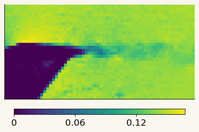
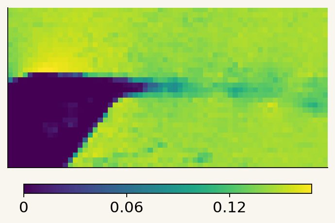
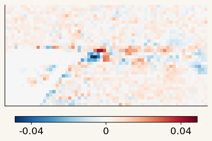
We repeat the last observed u/v channels at every input step. Earlier frames describe motion; the last frame anchors its current position. This is already part of T1.
y: future velocity · s: local fluctuation scale · r: residual. A zero residual predicts persistence.
Last observed
Measured future
Target residual
Local normalization and statistical features
Normalize each location by its recent mean and smoothed fluctuation scale. Feed those statistics back as channels, preserving the magnitude information.
Local mean μ
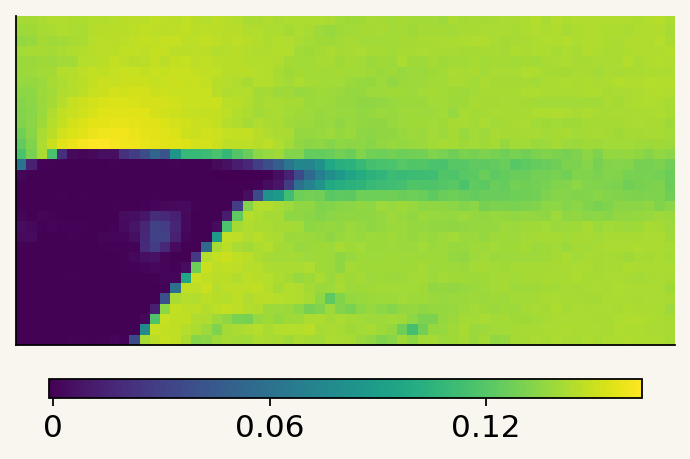
Fluctuation scale s
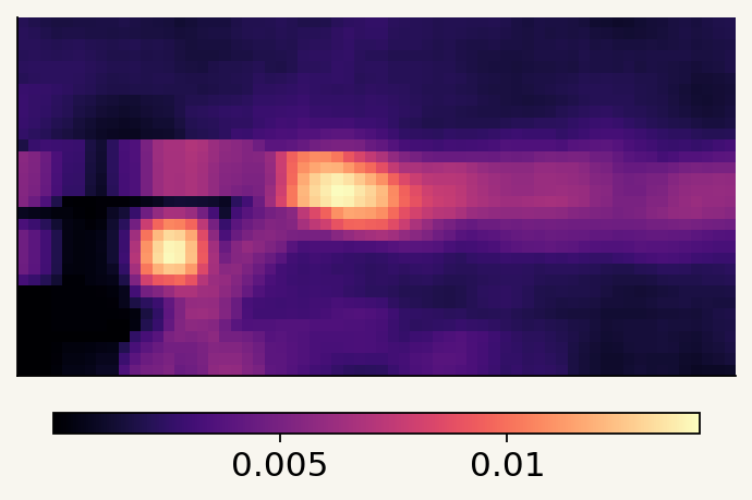
Normalized last frame
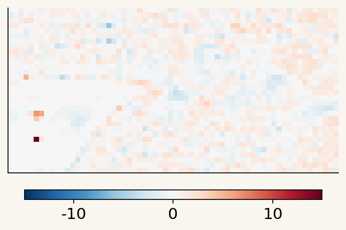
Keep scale available inside the network
Supplying scale channels at the input was one step. In the earlier U-Net, we also used local means and scales to modulate features after each InstanceNorm layer, through SPADE. That improved every scored component and supported the hypothesis that normalization was suppressing useful magnitude information. SPADE was a successful U-Net experiment; the final SimVP model retains the input statistics and local-scale residual decoding.
Experimental evidence and implementation
Residual targets and normalization are established forecasting tools; GraphCast uses normalized residuals. We combine them with repeated last-frame channels and flow-specific local statistics.
| Development experiment | Scoring version | Local quality |
|---|---|---|
| Within-window summaries, differences and global conditioning | v6 | 82.1980 → 82.4290 |
| Last-frame residual targets | v6 | 82.405 → 82.772 |
| Sliding temporal mean/MAD/STD | v9 | 79.2417 → 79.5046 |
| Local-scale normalization and residual decoding | v9 | 79.504625 → 79.868741 |
| SPADE after InstanceNorm, over a multiscale control | v9 | 79.869053 → 80.256412 |
The temporal-statistics change also improved the official Codabench final by 0.416149. In the subsequent validation diagnostic, observed fluctuation RMS and temporal-difference RMS had Spearman correlations of 0.962 and 0.966 with forecast-error RMS. Those associations motivated the local-scale experiment; they do not establish a causal effect by themselves.
These comparisons come from separate development stages. Scoring versions and some splits changed, so the gains are not additive. The repeated-last-frame concatenation comparison used different splits and has no isolated effect size. The early global conditioning and SPADE paths belong to the historical U-Nets.
The 18-channel stem combines u/v, last-frame u/v, sliding mean/MAD/standard deviation, window means, and log scales at 5×5, 3×3 and 9×9 neighborhoods. The plot uses a positive scale floor; training ties that floor to fitted channel statistics.
Real recording 10125_0.h5. Evidence: T1 METHOD §§2, 8.3–8.5; experiment ledger: history-conditioned point model, temporal statistics, observed-intensity diagnostic, and multiscale SPADE. Figure provenance.
What did removing features teach us?
Deleting the larger summary stack did not help the early model. A minimal input replaced temporal differences, summary maps and global conditioning with raw fields plus time/x/y coordinates: best local quality fell from 82.9800 to 82.4384. At a matched training budget, the full feature stack still performed better.
Removing the coordinates from that minimal model helped slightly, 82.4384 → 82.5063, while remaining below the full model. This supports testing which information is useful; it does not establish that coordinate removal would improve the full feature stack. These are historical v6 ablations.
Evidence: experiment ledger, “Minimal-input ablations” (4 August 2026).
02View augmentations
We introduced cropping to address the overfitting we observed.
The idea: vary the field of view so the model relies less on a fixed full-field layout and learns from local flow patterns.
Spatial cropping
25% of the area, used in 50% of samples. Native crops expose fine local structures. Full-field stride-two views preserve global context.
Move the crop. Inputs and targets keep the same coordinates.
Crop-size ablation

| Crop recipe | Best quality | Epoch | TKE |
|---|---|---|---|
| 80–100% area + resize | 81.8438 | 390 | 80.8037 |
| 40–70% area + resize | 81.9379 | 395 | 80.8813 |
| 25% area · native crop | 82.1057 | 380 | 81.3274 |
Same split, seed, base recipe and 400 × 800 updates. The milder crops resize with bilinear interpolation; the retained crop preserves native samples. This tests the full crop recipe, not area alone.
Our quarter-area crop removes much more context than the 80–100% and 40–70% resized crops we tested, yet gave the best validation result. It keeps native samples and alternates with full-field views.
Related work
Small crops are established in vision: Torchvision's RandomResizedCrop defaults to 8–100% of image area. Spatial cropping also appears in PDE representation learning, including Mialon et al. (NeurIPS 2023) and PIANO.
Our experiment tests native quarter-field crops as regularization for supervised velocity forecasting. The result supports this particular recipe; those earlier works study different objectives.
Same-recording mixup
Mix two non-overlapping windows from the same recording. One coefficient blends both inputs and targets.
Window A


Window B


Mixed


Inputs and targets advance together. The mixing weight stays fixed during playback. All panels share a speed scale: 0–0.172.
Vertical reflection
v′(row, col) = −v(H − 1 − row, col)
Original v

Image flip only

Flip + negate v

The same observed frames in all three panels. Blue: negative v. Red: positive v.
Augmentation settings & evidence
Mixup is established; selecting partners from the same recording keeps the flow condition consistent. T1 development quality was 82.054000 for same-recording mixing versus 81.983664 across recordings.
T2 mixes every sample using a folded Beta(0.5, 0.5) draw. The crop studies used mixup probability 0.5 and alpha 0.2. Full-field views sample all four stride-two spatial phases.
Crops and reflections stay aligned across inputs, targets and history maps. Reflecting v intervals also swaps their negated lower and upper endpoints.
Real recording 10125_0.h5 · Re 10,142 · AoA 0°. Figure provenance.
03Model architecture and training losses
Share most of the model. Give point prediction and uncertainty their own final block.
A sharp forecast and a useful uncertainty estimate need different features. Splitting late gives each objective capacity while keeping most computation shared.
Residual and fluctuation-energy losses
Selected T2 objective. TKE terms reward temporal fluctuation energy at two spatial scales.
Pixelwise error alone can favor smooth forecasts. Energy terms encourage the model to retain the flow's variation; quantile and SPS losses train the uncertainty bounds.
Architecture choices & experiment results
We build on SimVPv2/gSTA: spatial encoding, temporal translation and spatial decoding. Shared features with separate task heads follow a familiar multi-task learning pattern.
The first seven translator blocks are shared; the final gSTA block and decoder are separate. The point output is detached before the interval loss. Both objectives still train the shared backbone through their own paths.
| T1 development milestone | Local quality |
|---|---|
| SimVPv2 + joint SPS | 81.971903 |
| Cropping + 800 updates | 82.105752 |
| Dedicated late SPS path | 82.151385 |
These milestones summarize complete configurations. T1 also used an MVPE loss; the selected T2 recipe omitted it. Interval training combines quantile-style supervision with a smooth direct-SPS objective.
Evidence: T1 METHOD §§2, 4, 8; T2 METHOD §§2, 4–5. Quantile-based uncertainty background.
04Learning uncertainty
Learn bounds that adapt to the observed flow and reward useful precision.
Why we explored this. Our early calibration experiments showed that forecast errors carried structure: conditioning residual distributions on motion improved their bounds, and local spatial context helped further. The widest intervals covered more targets, yet did not earn the best SPS score. Those results supported two choices: let the input determine the uncertainty, and train for the score's balance between containing the target and keeping the interval narrow.
Let uncertainty depend on the flow
The first reference used one fixed residual interval per forecast horizon and velocity component. A small neighbor-aware convolutional model could instead use the local flow context to predict asymmetric bounds. We trained lower and upper residual quantiles, then calibrated them with conformalized quantile regression (CQR).
ŷ: point forecast · x: observed flow context · δ: learned lower and upper point-error offsets.
Train for useful bounds
SPS rewards intervals that contain the target while penalizing excessive width, with a multiplier for forecast accuracy. We kept quantile training and added a smooth approximation of this objective. Smooth interval-membership functions supplied gradients; evaluation still used the hard scorer. With the original inputs held fixed, direct-SPS training improved over CQR alone. Adding input-window summaries and a longer fit improved it further.
Early calibration experiments and what they showed
In the first benchmark, the point forecaster was frozen. Calibration used trajectory-group folds; the following are held-out validation results under the early v6 scoring protocol.
| Interval model | SPS | Coverage | Mean half-width |
|---|---|---|---|
| Constant per horizon/channel | 59.856 | 75.2% | 0.00941 |
| Neighbor convolution, Gaussian likelihood | 60.430 | 91.1% | 0.01857 |
| Neighbor convolution, asymmetric CQR | 61.257 | 89.7% | 0.01284 |
CQR improved local four-metric quality from 82.275 to 82.626 over the constant reference. It also beat the Gaussian head's SPS while using narrower intervals. A separate residual-histogram experiment found that motion conditioning supplied most of its gain, with spatial localization adding less.
The next comparison used a later fixed point checkpoint and a 20% calibration partition. It is a separate benchmark, also scored with v6.
| Width-24 interval head | Validation SPS |
|---|---|
| Original 13 inputs, CQR | 61.532 |
| Same inputs, 8 direct-SPS epochs | 61.903 |
| Full input summaries, 64 direct-SPS epochs | 62.210 |
| Full-input recipe, second seed | 62.211 |
The same-input comparison supports direct-SPS training. The full-input result combines richer features and a longer fit. These early v6 SPS values should not be compared directly with later v9 results.
Evidence: T1 METHOD §8.2; experiment ledger: frozen-forecaster calibration benchmark, local highest-density intervals, and direct SPS optimization.
Give uncertainty its own learned features
Later experiments trained the forecaster and interval head together, allowing uncertainty training to influence their shared representation. The final SimVP model carries this direction forward with a dedicated late SPS path, followed by learned interval refinement. The early standalone calibration heads were steps toward that design.
Joint-training result under the later scoring protocol
Under v9, a train-only CQR head on a frozen backbone scored validation SPS 42.7046 and local quality 78.4211. A joint model trained from random initialization reached 46.1662 SPS and 78.9916 quality. Calibration selected its epoch and validation remained untouched.
This compares training recipes, including their budgets and objectives. It supports the joint-training direction without isolating a single architectural change.
Evidence: T1 METHOD §8.4; experiment ledger, “Train-only SPS and end-to-end joint training” (9 August 2026).
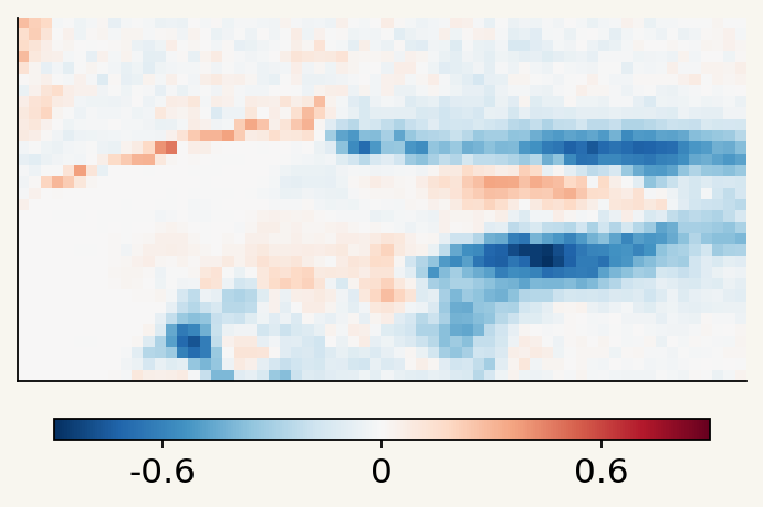
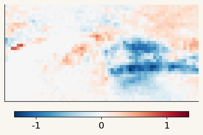
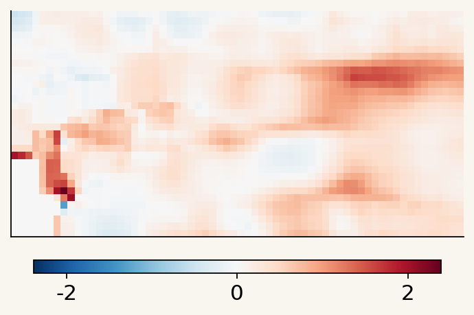
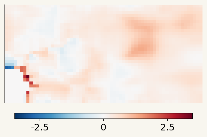
05T2 history features
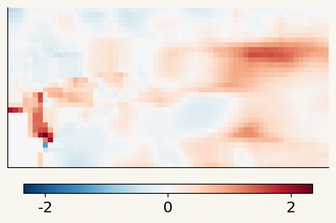
T2 adds seven maps from earlier observations to our strongest T1 architecture. The weights stay fixed.
The past tells us what is typical. Comparing it with the current window reveals shifts in mean flow, variability and fluctuation energy.
Mean shift · u
Mean shift · v
Log-scale shift · u
Log-scale shift · v
History confidence
Window energy · u
Window energy · v
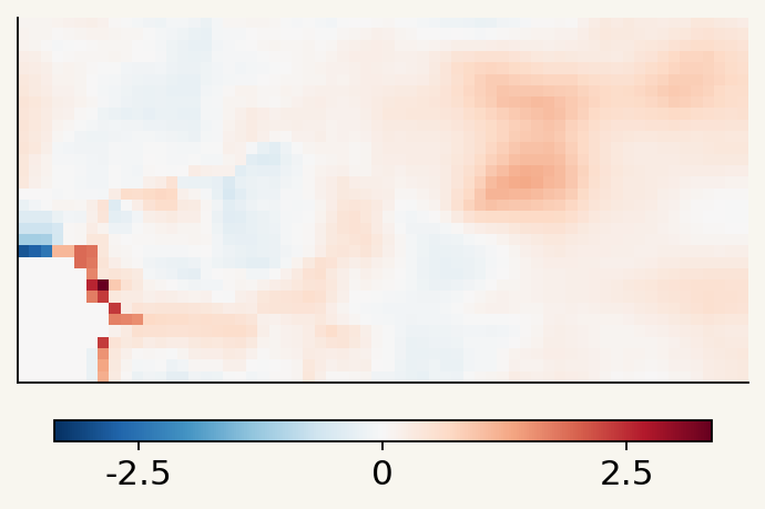
Actual feature maps: Re 25,482 · AoA 15° · 180 prior frames. Each map has its own scale.
A small projection adds 3,537 parameters—about 0.018% of the T1 model.
Feature definitions and validation results
Mean and log-scale channels compare the historical flow with the current window. The energy channels use average variance within completed windows, separating fluctuations from changes in window means.
Confidence grows with prior-frame count. Running sums keep memory fixed; state resets at recording boundaries. Future targets never enter it. Mixup uses the common prefix before both windows.
Running statistics are standard. The seven-map representation and its injection into the spatial stem are our design choices: a 7→32 linear convolution plus a 7→16→32 nonlinear path, initialized as a zero correction.
| Original package | Local quality | Velocity MAE |
|---|---|---|
| T1 | 82.509437 | 0.005760069 |
| T2 | 82.713986 | 0.005638215 |
+0.204549 quality; 2.115% lower MAE. This compares complete packages: T2 also changed mixup, precision, losses, checkpoint selection and PP caching.
Same 16 validation recordings and 653 windows. Evidence: T2 METHOD §§2–4, 6, 8. Figure provenance.
06Prediction postprocessing
Refine the forecast's energy and uncertainty with small learned correction networks.
Averaging predictions can smooth fluctuations. Four small KE networks correct the forecast; a width CNN adjusts uncertainty bounds and shifts.

Postprocessing methods and validation results
Native and vertically reflected inputs run as a packed pair. Mapping back reverses rows and negates v; interval endpoints swap under negation. At fixed T1 checkpoint weights, this TTA step improved quality 82.105752 → 82.188882.
The full correction stage combines midpoint blending, analytic fluctuation-energy corrections, four small KE networks, a width CNN and fitted width calibration. These are lightweight correction models, not four full forecasters.
| T2 pipeline | Before finishing stage | Final quality |
|---|---|---|
| Original submission | 82.485017 | 82.713986 |
| Fresh reproduction | 82.467032 | 82.708458 |
The original archive transferred PP from an earlier T2 model. The final training package freezes the new forecaster and fits fresh corrections on 65 optimization recordings, keeping the 16 validation recordings separate.
The figure shows final bounds, not a before/after comparison. Evidence: T1 METHOD §§5–8; T2 METHOD §§4–8.
07Inference optimization and reproducibility
We optimize neural inference, postprocessing and history updates together.
Mixed precision reduces neural computation. Graph replay reduces launch overhead. Running statistics keep history storage fixed as the recording grows.
Runtime details & reproduction evidence
CUDA Graphs and mixed precision are standard tools. We adapted the fixed-shape predictor, history updates and PP to work together under graph replay. Physical statistics and returned arrays stay FP32; returned predictions own their storage.
The offline Docker pipeline trains the forecaster, fits fresh PP, exports the model and checks the predictor interface. All learned components start from random initialization.
| T2 package | Local quality | Velocity MAE |
|---|---|---|
| Original submission | 82.713986 | 0.005638215 |
| Fresh reproduction | 82.708458 | 0.005650316 |
Training totaled 9h 38m 52s across two Colab sessions, including scheduled validation. PP cache generation, fitting and export took 25m 45s. These are measured stage durations, excluding downtime and recovery work.
Both evaluations use the same 16 recordings and 653 windows. Evidence: T2 METHOD §§7–9 and completed-run reports.
08What didn’t make the final model
The experiments we moved on from helped shape the final solution.
We explored alternative features, architectures, and augmentations, retaining changes that improved validation performance. We stopped some trials early, usually when their initial validation results did not justify further training. Several ideas improved training metrics or individual scores without improving overall forecast quality. The results below reflect the configurations and training budgets we tested.
Features
More explicit flow geometry. We tested whether giving the uncertainty model a solid mask, distance to the boundary, and vorticity and strain features would improve its error bounds. With the forecaster, folds, seed, and training budget held fixed, validation SPS fell from 61.293 to 61.116. Enlarging the neighborhood reduced it further, to 60.783. Coverage rose, but the intervals widened and their score fell. These particular extra features did not improve the uncertainty model.
Removing the derived features. We tested whether a simpler input would reduce overfitting. Removing temporal differences, local summaries, and global conditioning together lowered quality. A raw-only variant recovered a little by dropping coordinates, but still trailed the full feature stack. Adding an explicit half-cosine time channel to that minimal model also hurt. We retained the derived features.
Feature ablation results
These are early U-Net experiments under the v6 scoring protocol. They concern features derived from the current input window, separate from the longer recording history available in Track 2.
| Input recipe | Best local quality | What changed |
|---|---|---|
| Full feature stack | 82.9800 | Reference with differences, summaries, and global conditioning |
| Raw inputs + time/y/x coordinates | 82.4384 | Removed the derived feature bundle |
| Raw inputs only | 82.5063 | Also removed the coordinates |
| Raw inputs + half-cosine time | 82.4247 | Added time to the raw-only variant |
At a matched 6,000 optimizer steps, the full recipe led the raw-plus-coordinates variant, 82.8885 versus 82.3467. The feature-removal experiment tested the bundle as a whole; the coordinate and time-channel comparisons used the minimal model.
Evidence: experiment ledger, “Boundary-aware CQR ablation” and “Minimal-input ablations.” See what the model needs to see for the features we retained.
Architectures
Trying other forecasters. The search extended beyond SimVP: we trained a ConvNeXt U-Net, SwinUNETR, a SimVP model with a parallel Fourier/FNO adapter, and several wavelet, recurrent, and temporal-attention variants. The completed 400-epoch ConvNeXt, Fourier-adapter, and SwinUNETR runs reached local quality scores of 82.0299, 81.7435, and 81.3539. We continued developing the SimVP recipe used in the final submission.
Learning a second correction with WDNO. We tried a wavelet diffusion neural operator as a residual refiner, including joint training and a version on top of a frozen SimVP. The frozen-base experiment produced only tiny changes. In a later fine-tuning run, the best quality equaled the base forecast with the correction gate set to zero: the refinement was effectively disabled. We dropped this extra stage.
CNO3D. We trained a CNO3D model with a dedicated uncertainty path and stopped early after 11 epochs. Its best validation quality was 72.2276, reached at epoch 10.
Architecture results and training budgets
Scores are the best local validation quality without runtime. Epoch counts show training completed against the planned budget.
Completed
| Architecture | Epochs / budget | Best quality |
|---|---|---|
| ConvNeXt U-Net + dedicated uncertainty path | 400 / 400 | 82.0299 |
| SimVP + parallel Fourier/FNO adapter | 400 / 400 | 81.7435 |
| SwinUNETR, approximately 15M parameters | 400 / 400 | 81.3539 |
The Fourier trial used a parallel adapter within SimVP. ConvNeXt used 800 updates per epoch; the Fourier and SwinUNETR runs used 400.
Stopped early
| Architecture | Epochs / budget | Best quality |
|---|---|---|
| CNO3D + dedicated uncertainty path | 11 / 1,000 | 72.2276 |
| SimVP + Legendre multiwavelet translator | 105 / 400 | 80.0401 |
| SimVP + jointly trained WDNO refiner | 130 / 400 | 79.8104 |
| ConvTT-LSTM, approximately 15M parameters | 5 / 400 | 75.1754 |
| Small TAU | 405 / 600 | 81.6119 |
| gSTA + TAU concatenation | 260 / 400 | 81.3967 |
| PFGNet | 10 / 600 | 79.5431 |
Comparing WDNO refinement with its own base forecast
We stopped the frozen-SimVP/WDNO run after 390 of 400 planned epochs. Its best refined quality was 81.8078, versus 81.8123 for the base forecast evaluated alongside it. The largest positive difference during training was only +0.0046. We stopped the subsequent fine-tuning run after 65 of 100 planned epochs. Its best quality was 81.8525, equal to the base with a zero correction gate; none of its validation evaluations improved on the corresponding base.
Architecture trial summary, including training budgets, best checkpoints, and refinement comparisons.
Augmentations
Gaussian input noise. Adding noise at 1% of each recording's velocity standard deviation produced a misleadingly low training loss. The noise inflated the local temporal scale used for normalization, reducing the normalized velocity-MSE term without a matching validation improvement. Best quality was 81.55, about 0.3–0.4 points below the comparable clean run. We removed this augmentation.
Mixing across recordings and resizing larger crops. Broadening mixup to different recordings gave a slightly lower score than using windows from the same recording. Larger crops resized to the model's input grid also underperformed the small crop kept at native resolution. We retained the same-recording mixing and native-crop recipes.
Perturbing temporal Fourier modes. An earlier experiment varied the amplitudes of low-frequency temporal modes to regularize fluctuation energy while preserving mean flow. It slightly improved peak TKE and reduced the training–validation TKE gap, but best overall quality fell from 82.0878 to 82.0392. Improving the targeted diagnostic was not enough to improve the forecast's combined score.
Augmentation comparisons
| Experiment | Best local quality | Reference in that comparison |
|---|---|---|
| Mixup across recordings | 81.9837 | 82.0540, same-recording mixup |
| 80–100% area crop + resize | 81.8438 | 82.1057, native 25% area crop |
| 40–70% area crop + resize | 81.9379 | 82.1057, native 25% area crop |
| Temporal spectral augmentation | 82.0392 | 82.0878, earlier v6 control |
The crop runs shared a split, seed, and 400-epoch training recipe, varying crop area and resampling together. Mixup was disabled in the Gaussian-noise experiment. Spectral augmentation used an earlier v6 control, with separate checkpoints for its best TKE and best overall quality.
Evidence: augmentation ledger, “Full-trajectory Gaussian input noise” and “Mixup across all training trajectories”; experiment ledger, “TKE-targeted temporal spectral augmentation”; crop comparison results. See view augmentations for the retained transformations.
Team Pistachio · Built on SimVPv2/gSTA.